Here is a dump of all of my notes from the CalTech Devops PGC certificate, they aren’t in any particular order. I will only be posting from the courses I found more relevant:

There were 5 lessons in this course:

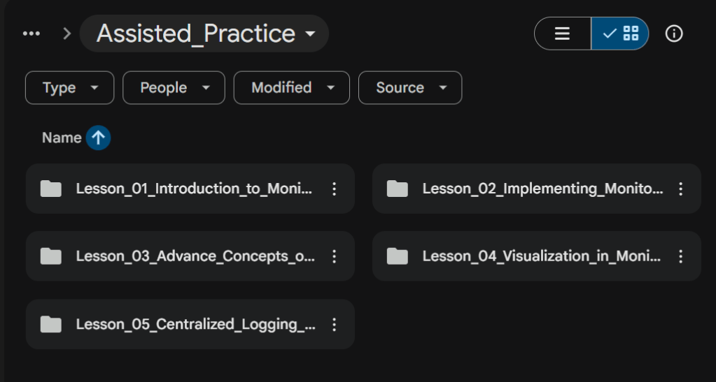
Lesson 01: Intro to monitoring
Setting Up Basic Infrastructure Monitoring Using Zabbix

This lesson demonstrates how to install, configure, and validate a complete Zabbix monitoring environment on Ubuntu. Readers begin by adding the Zabbix repository, installing the Zabbix server, frontend, agent, and required packages, then installing and enabling a MySQL database backend. The lesson walks through creating a dedicated Zabbix database and user, assigning permissions, and importing the Zabbix schema required for storing monitoring data.

Next, the lesson covers configuring the Zabbix server to connect to MySQL by updating the zabbix_server.conf file with the database password and restarting the required Apache, Zabbix Server, and Zabbix Agent services. Readers learn how to verify service status and ensure the monitoring platform is operational before proceeding to the web interface configuration.

The final section focuses on the Zabbix web console setup. Users access the Zabbix frontend through a browser, validate software prerequisites, configure the database connection, specify server settings such as timezone and theme, and complete the installation wizard. The lesson concludes by logging into the Zabbix dashboard using the default administrator credentials and exploring the monitoring interface, where infrastructure health, host availability, alerts, and performance metrics can be viewed and managed.

Configuring Prometheus to Scrape and Visualize Metrics

This lesson introduces Prometheus as a metrics collection and visualization platform. Readers begin by launching the Prometheus server from the command line using the provided prometheus.yml configuration file. The exercise emphasizes that the Prometheus service must remain running in the terminal for the web interface to function properly. Once started, the Prometheus server becomes accessible through its web interface on port 9090.

The lesson then explores the Prometheus Expression Browser, where users search for metrics and execute queries. A demonstration uses the process_virtual_memory_bytes metric to display memory utilization data collected by Prometheus. Readers learn how to execute PromQL queries and switch between tabular and graphical views to visualize performance metrics over time, providing immediate insight into application and system behavior.

Finally, the lesson explains how to validate metric collection by examining the Targets page within the Prometheus Status menu. Users verify that monitored targets are in the UP state and review scrape information, including last scrape times and errors. The exercise concludes by accessing the /metrics endpoint directly, allowing readers to view the raw metrics exposed by Prometheus and gain a deeper understanding of how monitoring data is collected and made available for visualization and analysis.

Lesson 02: Implementing monitoring with Prometheus

Setting Up and Monitoring with Node Exporter

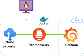
This lesson introduces Node Exporter, a Prometheus exporter that collects operating system and hardware metrics from Linux hosts. The exercise begins by downloading the Node Exporter binary, extracting the package, organizing the files into a dedicated directory, and launching the exporter as a background process. Readers verify successful operation by accessing the /metrics endpoint and viewing the raw system metrics exposed by Node Exporter.

The lesson then demonstrates how to configure Prometheus to scrape Node Exporter metrics. Users create a custom Prometheus configuration file containing a scrape job that targets the local Node Exporter instance on port 9100. After saving the configuration, Prometheus is started using the new YAML file, enabling automated collection of host-level performance metrics such as CPU, memory, disk, and network statistics.

The final section focuses on validating data collection through the Prometheus web interface. Readers access the Prometheus UI, query metrics such as node_cpu_seconds_total and node_memory_Active_bytes, and view graphical representations of system performance. The lesson concludes by checking the Targets page to confirm that the Node Exporter target is healthy and being successfully scraped by Prometheus.

Writing Basic Queries in PromQL

This lesson introduces Prometheus Query Language (PromQL) and demonstrates how to retrieve, filter, aggregate, and manipulate monitoring data. Readers begin by launching Prometheus and accessing the Graph interface, where they execute a simple query against the node_cpu_seconds_total metric to view raw CPU statistics collected from monitored systems.

The lesson then explores filtering metric data using labels. Users query filesystem metrics such as node_filesystem_avail_bytes and narrow results by specifying label values like device names. This demonstrates how PromQL enables precise selection of individual time series from a larger dataset. Additional exercises show how to aggregate metrics using functions such as sum() and perform arithmetic operations to convert values into more meaningful units, such as displaying memory availability in megabytes rather than bytes.

Finally, readers learn to calculate rates using the rate() function. By applying rate(node_network_receive_bytes_total[1m]), they determine the average per-second network receive rate over the previous minute. The lesson concludes by emphasizing how PromQL enables efficient analysis of system performance and operational trends through flexible querying capabilities.

Writing Advanced Queries for Real-Life Use Cases

This lesson expands on basic PromQL concepts by applying advanced queries to practical monitoring scenarios. The first exercise focuses on memory utilization monitoring. Readers execute a query that calculates memory usage as a percentage of total system memory, allowing administrators to identify nodes approaching resource exhaustion and create alert thresholds for proactive response.

The lesson then demonstrates infrastructure performance analysis through disk I/O monitoring. Using PromQL rate functions and aggregation operators, users calculate read and write throughput across systems and group results by instance. This helps identify abnormal disk activity patterns, bottlenecks, and storage-related performance issues that may impact applications.

Additional exercises focus on operational visibility and maintenance planning. Readers calculate node uptime by comparing system boot time with current system time, converting the result into days to identify systems that may require maintenance or reboot scheduling. The lesson concludes by monitoring network traffic rates to detect potential bottlenecks, demonstrating how advanced PromQL expressions can provide actionable operational intelligence for performance management and alerting.

Writing PromQL Queries to Extract Specific Metrics from a Sample Dataset

This lesson demonstrates how to use PromQL to extract targeted information from Node Exporter metrics collected by Prometheus. The exercise begins by deploying a complete monitoring environment using Docker and Docker Compose. Readers clone a Prometheus playground repository, configure Node Exporter and Prometheus containers, adjust port assignments to avoid conflicts, and verify that both services are running successfully.

After the environment is operational, users access the Prometheus UI and begin querying Node Exporter metrics. The lesson introduces label-based filtering by querying CPU statistics such as node_cpu_seconds_total{mode=”system”} to isolate CPU time spent in system mode. Readers then refine queries further by filtering on specific CPU cores and using regular expressions to match multiple label values dynamically. These exercises demonstrate how labels provide granular control over metric selection.

The lesson concludes by showing how PromQL can combine multiple filtering techniques to extract meaningful operational data from large metric datasets. By selecting metrics based on names, labels, and pattern matching, readers gain practical experience building targeted monitoring queries that support troubleshooting, performance analysis, and infrastructure observability.

Lesson 03: Advanced concepts with Prometheus monitoring

Adding Instrumentation to a Java Application

This lesson demonstrates how to instrument a Java application so that Prometheus can collect and visualize application metrics. The exercise begins by cloning a sample Java application from GitHub and navigating to the java_simple project directory. Git must be installed before proceeding.

The lesson then uses Maven to build the application into an executable JAR file. After a successful build, the application is launched in the background using Java. Verification is performed by accessing localhost:1234, which returns a “Hello World!” response. Readers also confirm that the application exposes Prometheus metrics through the /metrics endpoint.

Next, Prometheus is configured to scrape the application’s metrics by creating a java-metrics.yaml configuration file. A scrape job named my-java-app targets localhost:1234 and collects metrics from the /metrics endpoint. Prometheus is then started using this configuration file.

Finally, readers use the Prometheus web interface to visualize application metrics. Queries such as hello_worlds_total and jvm_memory_bytes_committed are executed to observe metric values and graph trends. By repeatedly accessing the application, users can see counters increase in real time, demonstrating successful instrumentation and monitoring of a Java application.

Configuring Alertmanager for Email Notifications

This lesson focuses on integrating Prometheus with Alertmanager to provide automated email notifications when monitored systems experience issues. The process begins by creating a Prometheus configuration file that defines Alertmanager as the alerting endpoint and references a rules file containing alert definitions. Prometheus is configured to monitor both itself and Node Exporter.

The lesson then creates a rules.yml file containing an InstanceDown alert. This rule triggers whenever a monitored target becomes unavailable for more than one minute. Alert metadata, including severity levels and descriptive annotations, is included to provide meaningful notification content.

Next, Alertmanager is installed and configured. A custom configuration file specifies Gmail SMTP settings, sender and recipient email addresses, routing behavior, notification grouping intervals, and receiver definitions. Alertmanager is then launched as a background service to handle notifications generated by Prometheus.

The final portion validates the alerting workflow. Node Exporter and Prometheus are started, and the Prometheus Alerts page is reviewed. To simulate a failure, the Node Exporter process is manually terminated, causing the InstanceDown alert to transition from inactive to active. Users then verify that Alertmanager receives the alert and displays the same status through its web interface, confirming successful end-to-end alert processing and notification delivery.

Automating Metric Pushing with a Cron Job

This lesson introduces Pushgateway and demonstrates how short-lived jobs can push metrics to Prometheus through automated scripts and scheduled tasks. The exercise begins by downloading and extracting the Pushgateway binary, removing the installation archive, and launching Pushgateway as a background service. Users verify successful startup by accessing the Pushgateway web interface and reviewing runtime information.

The lesson then configures Prometheus to scrape Pushgateway metrics. A custom prom-pushgateway.yml file is created with a scrape job targeting localhost:9091, the default Pushgateway port. Prometheus is started using this configuration, and users verify that the Pushgateway target appears in the Prometheus Targets dashboard.

Next, a Bash script is created to generate and push custom metrics to Pushgateway. The script formats metrics according to the Prometheus exposition format and sends them to Pushgateway using HTTP requests. This approach enables short-lived processes, which cannot be scraped directly by Prometheus, to expose metrics for later collection.

The lesson concludes by automating script execution with a cron job. Metrics are pushed at scheduled intervals, and users verify successful operation by viewing the metrics in Pushgateway and querying them through the Prometheus UI. This workflow demonstrates how cron jobs, Pushgateway, and Prometheus work together to provide monitoring visibility for batch jobs and ephemeral workloads.

Lesson 04: Visualization in monitoring using Grafana

Setting up a Grafana Instance

This lesson walks through installing Grafana on a Linux system using the official APT repository. The process begins by installing prerequisite packages, importing Grafana’s GPG key, adding the Grafana repository to the system’s APT sources, and updating the package list. The lesson also covers resolving potential repository key conflicts that may occur during installation.

After the repository is configured, Grafana is installed using the package manager. The Grafana service is then started using systemctl, and its status is verified to ensure that the service is running correctly. Readers are instructed to reload the system manager configuration before starting the Grafana server.

The final portion focuses on accessing the Grafana web interface through http://localhost:3000. Users log in using the default administrator credentials and are prompted to change the default password. Upon successful login, the Grafana dashboard becomes available for future monitoring and visualization tasks.

Building a Multi-Panel Dashboard in Grafana

This lesson demonstrates how to integrate Prometheus with Grafana and create dashboards for monitoring infrastructure metrics collected through Node Exporter. The exercise begins by logging into Grafana and adding Prometheus as a data source. Users configure the Prometheus URL (http://localhost:9090) and validate the connection using Grafana’s “Save & Test” feature.

Once Prometheus is connected, a dashboard is created by importing a pre-built Grafana dashboard template. The lesson uses dashboard ID 1860, a commonly used Node Exporter dashboard, which provides multiple panels for monitoring server performance metrics. Users select the Prometheus data source and import the dashboard into Grafana.

The imported dashboard automatically generates multiple panels displaying infrastructure metrics such as CPU utilization, memory consumption, disk usage, network activity, and other system performance indicators. Individual panels can be expanded for more detailed analysis, allowing administrators to compare resource utilization across servers from a centralized dashboard.

Configuring Email Alerts for Critical System Thresholds

This lesson explains how to create automated email notifications in Grafana when monitored systems exceed predefined thresholds. The process starts by generating a Gmail App Password, which provides secure authentication for Grafana’s SMTP integration. The lesson explains how to create, use, and later remove the app password for security purposes.

Next, Grafana’s SMTP configuration is updated by modifying the grafana.ini file. SMTP settings such as the Gmail server address, user account, app password, sender address, and sender name are configured. Grafana is then restarted to apply the changes.

After email functionality is enabled, users create a Contact Point within Grafana’s Alerting section. Email addresses are specified as notification recipients, and test notifications are sent to verify that SMTP integration is functioning correctly. Once validated, the contact point is saved for future alerting workflows.

The lesson concludes by configuring notification policies and alert rules tied to Prometheus metrics. When monitored values exceed critical thresholds, Grafana automatically generates and sends email alerts to designated recipients, providing proactive notification of system issues.

Creating a Grafana Dashboard Using PromQL Queries to Visualize Specific Application Metrics

This lesson focuses on building custom Grafana visualizations using PromQL queries against Prometheus metrics. Users begin by logging into Grafana, creating a new dashboard, and adding a visualization panel. Prometheus is selected as the dashboard’s data source, making all collected Prometheus metrics available for visualization.

The lesson then creates a CPU Usage panel using a Time Series visualization. Users access the query editor, switch to code mode, and enter a PromQL expression that calculates CPU utilization based on Node Exporter metrics. The panel is configured with a descriptive title and executed to display live metric data.

By applying the visualization to the dashboard, users create a reusable monitoring panel that provides real-time insight into system performance. The exercise demonstrates how Grafana and PromQL work together to transform raw Prometheus metrics into meaningful visual dashboards that can be customized for specific operational requirements.

Setting up Docker Monitoring Using Prometheus and Grafana

This lesson demonstrates how to deploy a complete container monitoring solution using Docker, Prometheus, Grafana, and cAdvisor. The process begins by creating a working directory, cloning a preconfigured monitoring repository from GitHub, and launching the monitoring stack using Docker Compose. The stack automatically deploys Prometheus, Grafana, Alertmanager, Node Exporter, and cAdvisor containers.

After deployment, users verify that cAdvisor is exposing Docker metrics through the /metrics endpoint. cAdvisor provides detailed visibility into container resource consumption, including CPU, memory, storage, and network utilization. The lesson also provides troubleshooting guidance for resolving port conflicts if services fail to start.

Next, users access the Grafana dashboard that accompanies the monitoring stack. The dashboard contains separate sections for host-level metrics and container-level metrics. Host monitoring includes uptime, memory usage, disk utilization, load averages, network activity, CPU usage, and disk I/O. Docker monitoring focuses on per-container CPU usage, memory consumption, swap usage, and network statistics. Alerts are configured to warn administrators when critical thresholds are reached.

The lesson concludes by launching additional Docker containers and observing how the Grafana dashboard updates automatically. Newly created containers appear within the monitoring panels, demonstrating real-time visibility into containerized workloads and validating the complete monitoring pipeline.

Lesson 05: Centralized logging and monitoring

Setting up and Configuring Elasticsearch for Log Storage

This lesson demonstrates how to deploy Elasticsearch as a centralized repository for application logs. The exercise begins by verifying that the Elasticsearch service is operational using a simple HTTP request against port 9200. This confirms that the cluster is accessible and ready to receive data.

The lesson then walks through creating an Elasticsearch index named my-index using a PUT request. During index creation, users define shard and replica settings as well as mappings that specify data types for indexed fields. This demonstrates the importance of planning storage structure and search behavior before ingesting data.

After creating the index, a sample document is inserted using a POST request. The document contains fields such as field1 and field2, illustrating how structured data can be stored and indexed within Elasticsearch. Users then verify index creation and document storage by listing indices and retrieving the document directly from Elasticsearch.

The lesson concludes with index cleanup procedures. Once validation is complete, the index is deleted and the system is checked to confirm successful removal. Through this process, users gain practical experience with index creation, document insertion, retrieval, verification, and deletion while learning how Elasticsearch supports scalable log storage and search capabilities.

Building Logstash Pipelines for Centralized Log Collection

This lesson focuses on configuring Logstash to ingest, process, and forward log data into Elasticsearch. The process begins by creating a Logstash pipeline configuration file that contains input, filter, and output sections. Logstash is configured to accept standard input, optionally process data through filters, and send events to Elasticsearch while simultaneously displaying output in the console using the Ruby Debug codec.

Once the pipeline is configured, users manually start Logstash and test connectivity to Elasticsearch. Sample log data is entered into the Logstash console, where it is immediately processed and forwarded to Elasticsearch. The lesson demonstrates how Logstash serves as an intermediary layer responsible for collecting, transforming, and routing log events.

Verification steps include confirming the creation of a test_index within Elasticsearch and querying the index contents to ensure that the log message was successfully stored. This provides validation that the complete data pipeline—from ingestion through indexing—is functioning properly.

By completing this exercise, users learn how Logstash pipelines centralize log collection, simplify log processing workflows, and enable efficient storage and analysis of operational data within Elasticsearch.

Building Dashboards and Visualizations in Kibana

This lesson demonstrates how Kibana transforms raw log data into searchable visual insights. The exercise begins by launching Logstash and generating sample application logs containing various severity levels such as DEBUG, INFO, WARN, ERROR, and FATAL. These logs are indexed into Elasticsearch and serve as the data source for visualization.

After validating that the logs have been stored in Elasticsearch, users access the Kibana web interface through port 5601. The lesson guides users through Kibana’s initial setup process, including navigating the dashboard, exploring logs, and accessing Stack Management to configure data views.

A data view is then created to connect Kibana with Elasticsearch indices. Once configured, users explore log records through the Discover interface, where indexed events become searchable and filterable. This enables administrators to quickly investigate system behavior and identify operational issues.

The final portion of the lesson focuses on visualization creation. Users select log fields, build visualizations, and generate stacked bar charts that display log statistics and trends. These dashboards provide valuable operational visibility, helping teams monitor application performance, detect anomalies, and troubleshoot issues more effectively.

Building an Automated Log Processing Pipeline with Kafka and the ELK Stack

This lesson introduces a scalable log-processing architecture that integrates Apache Kafka with the ELK Stack. The objective is to buffer log traffic through Kafka before forwarding it to Logstash and Elasticsearch, thereby protecting downstream components from traffic spikes and improving reliability during high-volume logging events.

The setup begins by preparing the Linux environment, updating system packages, and installing the Java Runtime Environment required by Kafka and related components. Elasticsearch repositories and signing keys are configured to support installation and updates of ELK Stack components.

Next, a Logstash pipeline is configured to consume messages from a Kafka topic named apache. Logstash uses a series of filters—including Grok parsing, date processing, and GeoIP enrichment—to transform raw Apache log entries into structured records suitable for indexing and analysis. Processed events are then sent to Elasticsearch for storage.

The lesson also includes installation and configuration of Apache HTTP Server and Filebeat. Filebeat is configured to monitor Apache access logs and publish them directly to Kafka. Kafka acts as the message broker, decoupling log producers from consumers and providing resilience during periods of increased log volume.

Together, Filebeat, Kafka, Logstash, Elasticsearch, and Kibana form a complete enterprise-grade log analytics platform. The architecture enables reliable log ingestion, buffering, parsing, enrichment, storage, visualization, and long-term observability for modern applications and infrastructure.